Sieve Analysis Test Report

 CONSTRUCTION REPORT 1:  SIEVE ANALYSIS

 (CONSTRUCTION LAB)

Introduction:

The objective of this experiment consists in determining the particle size distribution of fine and coarse aggregates to find soil properties by a soil analysis. We use 12 sieves of different diameters, a brush, a balance, and soil.

Description of the apparatus:

Experimental procedures:

1) Use the brush to clean all the sieves.

2) Determine the mass of each sieve without soil.

3) Place the sieves with openings of decreasing size from top to bottom (a pan is placed below the stack).

4) Determine the mass of soil sample = the mass of (soil+ sieve) – the mass of sieve.

5) The soil then is shaken through the stack of sieves

6) After the soil is shaken, the mass of soil retained on each sieve and in the pan (Mp) is determined.

Theoretical basis:

1) Determine the total mass of the soil: M1 + M2 · · · +Mn + Mp = M

2) Determine the cumulative mass of soil retained above each sieve. For the I’th sieve, it is M1 +M2 +.  · · + Mi

3) The mass of soil passing the I’th sieve is M = (M1 + M2 +· · · +Mi)

4) The percent of soil passing the I’th sieve (or percent finer) is F= [ M-( M1+ M2 +…. +Mi)] *100/M

5) The calculations are finally plotted on semi-logarithmic graph paper

Data collection and calculation:

Mass of soil sample = 1052g

Sieve opening (mm)	Mass of sieve (g)	Mass of soil + sieve (g)	Mass of soil retained (g)	Cumulative mass retained (g)	%Retained	%Passing
50	612	612	0	0	0	100
37.5	556.5	556.5	0	0	0	100
25.4	577.5	595	17.5	17.5	0.37	99.63
25	559.5	571	11.5	29	0.58	99.42
12.5	602.5	2171	1568.5	1597.5	31.95	68.05
4.75	575	2197	1622	3219.5	64.39	35.61
2	534	616	61.5	3281	65.62	34.38
1.18	493	535	42	3323	66.46	33.54
0.85	487	538	51	3374	67.48	32.52
0.425	452	873	421	3795	75.9	24.1
0.15	424.5	1500	1075.5	4871.5	77.43	22.57
0.075	415.5	522	106.5	4977	99.54	0.46
pan	468.5	491	22.5	4999.5	99.99	0.01

Draw the graph using log 10 scale for the x axis:

On log paper:

Now, find D60, D10, D30, D75, and D25 and use them to calculate different coefficents needed for soil classification.

D60: the 60% finer size = 10

D10: the 10% finer size = 0.1

D30: the 30% finer size = 0.96

D75: the 75% finer size = 42

D25: the 25% finer size = 0.92

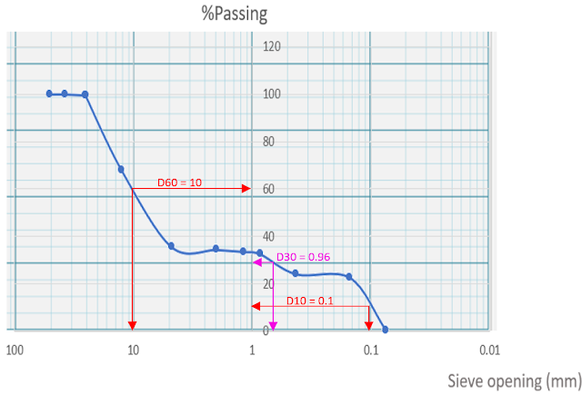
Uniformity coefficient: Cu = D60 / D10 = 10/0.1 = 100

Coefficient of gradation: Cc = (D30) ^2 / (D60*D10) = 0.96^2/ (10*0.1) = 0.9216

Sorting coefficient: S0 = (D75/ D25) ^0.5 = (42 / 0.92) ^0.5 = 6.756

Based on the graph shape, and on the coefficients, we can determine the size distribution of the aggrigates in the soil.

As we can see, our aggregates are gap- graded, based on the shape of the graph.

In this image, we can see the distribution of aggrigates in different soil type.

At last, the soil is classified using the following rules:

• If Cu < 2: uniform graded soil
• If Cu > 4 and Cc is in between 1 and 3: well-graded gravel else poorly graded or gap graded gravel
• If Cu > 6 and Cc is in between 1 and 3: well-graded sand else poorly graded sand.

This measure tends to be used more by geologists than engineers. The larger So, the more well−graded the soil.

For well−graded soils, Cc~ 1.

Soils with C u <= 4 are considered to be "poorly graded" or uniform.

The "effective size" of the soil: D10.

Empirically, D10 has been strongly correlated with the permeability of fine−grained sandy soils.

References:

 1)       Construction lab (BAU)

2)        Book: principles of geotechnical engineering (25th edition)